How To Create A Six Sigma Control Chart In Excel?
The Six Sigma control chart is a simple but effective method for determining process or organizational reliability over time. A graph that covers a time span, a centerline that shows the effects of an operation during that time, and upper and lower control limits showing whether the process variance is within the agreed range involves the purpose of control charts. A tracking diagram includes a means of detailing a process and enhancing it, and a diagram showing the effects. This is critical because processes fall under four states: optimal, ideal, chaotic, and messy threshold. This is crucial knowledge.
An inspection diagram is a way to take the information to build and develop a process and to provide a diagram that displays the results. This is valuable knowledge because processes fall under four states: optimal, ideal threshold, on the verge of chaos and chaos.
So many companies, before reforming, wait until the last.
What is a Control Chart in Excel?
We actually have differences everywhere, no mechanism is unchanged. This means that no variation or variation of the trigger will occur frequently. In the control charts, we see how these changes influence our process over a certain time, whether our processes are under control or transcend process limits. Check diagrams allow us to see this difference. Tables have a central or average line and the Upper Control Limit (UCL) and Lower Control Limit are available in our control table (LCL). The upper and lower control limits on both sides are 3 standard distance from the centre line.
The upper alarm line and lower warning limit can also be used. Now, this is the standard two-way deviation from the central line? The one that alerts us if data points cross this boundary can unstable the process.
How to Work with Control Chart in Excel ?
One concept may sum up the control chart excel template: All processes appear to gravitate to a state of chaos.
Any method or procedure, from the factory floor to a front desk at a hospital to your home office, will inevitably go into chaos without helping the hand of continuous process improvement and analysis. It’s just a question of time.
Just as a value map defines each phase of a process and specifies where mistakes and consistencies lie, a control panel provides a way of deciding whether the entire process leads to the best possible outcome.
This is achieved by calculating variance. Two classes are used in all combinations. Common cause variation – a mechanism is intrinsic to this form of variation. Variation of the common cause is predicted but is normally within control limits. This form of variation is random – there are no acts by a single individual or combinations of factors which lead to variation.
Shift in the special causes
This kind of variation is non-alleged and arises by a person’s actions or a combination of factors. The defects or process structures that can be corrected or replaced are badly planned.
Valuable knowledge is available to know the type of variance in a method. A diagram shows which form of variation exists. It helps you to understand when and when to act, and whether a process is at hand or on the verge of chaos.
Designing Control Chart
Setting up the control chart centerline allows you first to decide the data you need to chart.
A simple instance: every day you want to work on time. The centerline displays the time per day you got to work for a period of time. The centerline could represent the amount of sales achieved in a quarter for companies. The time it takes for a doctor to admit a patient to be registered.
You must then set control limits which indicate an appropriate range of differences. In other words, what is the predicted common explanation, the intrinsic random variation? This is calculated by the addition of data over a long period.
Using the basic example of working, you could calculate a time that is ten minutes late and ten minutes early, a time interval that takes into account the random changes in a commute. That is, automobile collisions, heavy-duty drivers, jams at certain areas, etc.
In detail on Control Charts
This provides a description of the operation of a control map. Control charts may provide charts of subgroup processes which are part of a final product for more complicated business activities.
For starters, thousands of components and jobs include building cars, trucks and aeroplanes. It might be appropriate to draw a diagram to chart subgroups such as building individual pieces.
It is necessary to bear in mind the following when creating a control chart:
- Collect and document production order data
- Collect data over a period to help you assess the top and bottom ranges of control by average
- Draw and connection points that indicate data over a period of time from left to right
- Take action on the diagram
This last segment is one of the most significant. Changes and patterns do not arise at random. A change is a change that unexpectedly reaches seven (7) points. A pattern is seen when seven points in a row shift in a direction up or down.
Steps involved in creating Six Sigma Control Chart in Excel
- Make sure the data is well displayed in one column. We believe that the data is worth 30 days for this tutorial and is present in a worksheet called ‘Control Map’ in the first column from cell A1 to A0.
- We often use the called range feature when generating the various series in the control chart. (Please learn more about building a name range map here.)
Now, in the menu, click ‘Insert’ -> ‘Name’ -> ‘Set.’ The “Insert Name” dialogbox will be opened as seen in the following image.
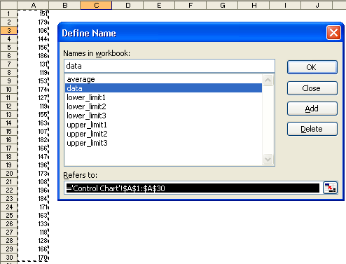
As you can see, the named range of the sequence, mean or average, you can also add upper and lower contrl limits in the control chart.
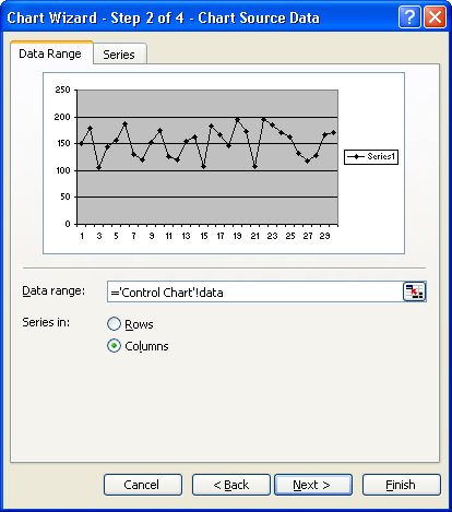
3. Insert a map with the option ‘Insert’ -> ‘Chart.’ Insert the “data range” as = “Control Data” in the ‘Chart Source Data’! Info. – Data. (We would have normally entered the source data range as ‘Control Chart’!$A$1:$A$30, but we’ll use it since we’ve built a named range that refers to it.)
4. Shape the diagram and delete ‘chartjunk.’ Right click and choose ‘Source Info’ from the map. Click on the ‘Add’ button and insert new statistical control limits in the average, lower, and higher serial.
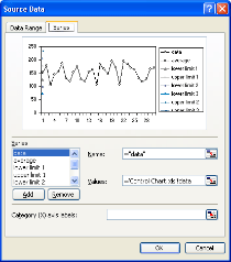
5. Shape the diagram and delete ‘chartjunk.’ Right click and choose ‘Source Info’ from the map. Click on the ‘Add’ button and insert new statistical control limits in the average, lower and higher serial.
The series we have introduced in point 4 are all shown in the chart as points. You can now select “Chart Type” one after one right click on any point, and change the type to XY Scatter in the box that appears. (Shortcut – You should do this once for the first point, then just pick the point and press F4 for the following points.)

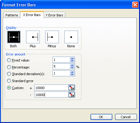
6. Once Step 5 is over double-click every point and pick the tab for the X Error Bars. Enter a reasonably high number of + and – errors in the custom error box (say 10000). For all the sequences, repeat this step except one that represents the main data.
7. The control chart tends to be like the one shown below once we have completed with points 1 to 6. His smooth sailing from this stage onwards.
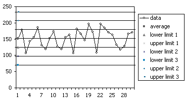
8. Click right on the map and pick the options ‘Chart.’ Enable the ‘Series Name’ and the ‘Value’ tab on the ‘Data Labels’ tab. Okay….bear to me….this IS a crazy looking control map, but there’s salvation.

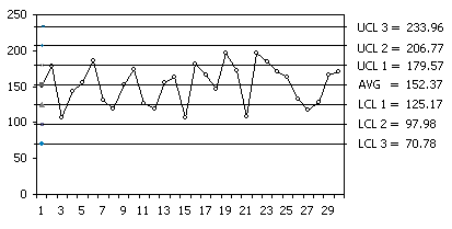
9. Click any of the labels of the key data series carefully in the Control Chart (the one that represents the data being plotted). Click to remove. This leaves all remaining series only with the value and series name. Choose a mark now. (Two subsequent clicks on the same mark slowly). Move the mark to the far right. Place all other labels by pressing F4. Pick each of them.
Click on the chart right and choose ‘Source Info.’ One by one, change and give a descriptive name to each of the series’ ‘Names.’ LCL1, LCL2, LCL3, UCL1, UCL3, UCL3 and AVG have been used for this. You must type the name in the following format.

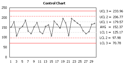
10. Only right-click one at one point and choose ‘Format Data Sequence.’ Monitor limits of the chart and the average. Set ‘Marker’ to zero in the ‘Patterns’ options window. Now click on each line and give the bands the right shading. We use light shades for broader control limits and darker shades to meet external and vital quality control constraints in our example. When you add 3 limits labels (+/- 1, 2, and 3), you have a six sigma regulation chart to make it the right one.
This content piece will surely help you in understanding how to create a control chart dashboard in QI.